Antenna Design, Monopole Antenna

I. Theory

1. Monopole Structure

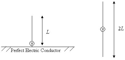
Figure: A monopole antenna (left) versus a dipole antenna (right)

- Lower half arm of the dipole is replaced with a perfect electric conductor (PEC).

- It is also called an antenna ground plane.

- A device case or platform often serves as an antenna ground plane.

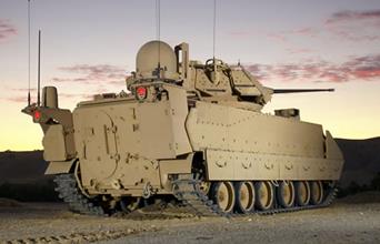
Figure: A device case or chassis can be used as an antenna ground plane.

2. Image Theory

Figure: Image principles.

- Find the field due to a current radiating above an infinite PEC ground plane

- Remove the PEC ground plane.

- Place an image current.

- The field above the ground plane is a sum of the fields due to the current and its image.

- The field below the ground plane is zero.

3. Monopole Impedance and Radiation Pattern

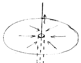
Figure: Current on a monopole fed by a coaxial cable.

- The current on the ground plane flows in the radial direction.

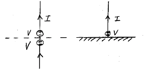
Figure: Voltage and current on a dipole (left) and a monopole (right)

- Input impedance of a monopole is one half of the dipole input impedance.

Figure: Directivity patterns of a dipole (blue) and a monopole on an infinite ground plane (red)

- Directivity of a monopole on an infinite ground plane is twice that of a dipole.

Figure: Relative directivity patterns of a monopole on an infinite ground plane

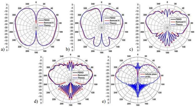
Figure: Normalized directivity patterns of a quarter-wave monopole on a circular ground plane of radius a. (a) a = 1λ, (b) a = 2λ, (c) a = 6λ, (d) a = 10λ, (e) a = 20λ. From Z. Zivkovic et al., "Radition pattern and impedance of a quarter wavelength monopole antenna above a finite ground plane", Proc. IEEE 20th Int. Conf. Software, Telecomm. Comp. Networks, 2012, pp. 1-5.

- Even with a large ground plane, it is difficult to completely block the field in the lower hemisphere.

- In the above figure, with a 40-λ diameter ground plane, the field behind the ground plane is reduced by only 9 dB.

4. Various Forms of The Monopole Antenna

4.1 Sleeve Monopole

- Enclose the base of the monopole with a conducting cylinder.

- Banwidth is greatly increased.

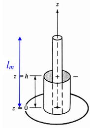
Figure: Sleeve monopole structure. From W. L. Week, Anenna Engineering, McGraw-Hill, 1968.

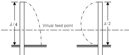
Figure: Principles of the bandwidth extension in the sleeve monopole

- Sleeve can be of open type.

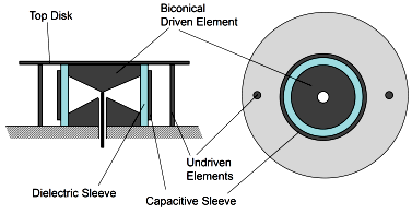
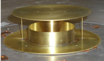
Figure: A cross-T-wire top-loaded open-sleeve monpole. Dimensions (in λ): driven element 0.13, top-loading element 0.035, sleeve 0.09-0.11 (tuning), driven element to sleeve 0.049, wire radius 0.0075. From L. J. Ying and G. Y. Beng, "Characteristics of broadband top-loaded open-sleeve monople", IEEE AP-S Int. Symp. Dig., 2006, pp. 635-638

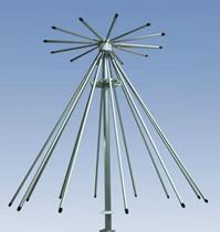
4.2 Monpole with Radials

- Groun plane is realized usign quarter-wave radials.

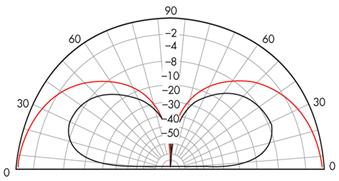
Figure: A monopole with radials (left) and its directivity pattern (right). From www.kingscountyradioclub.com

Figure: A VHF monopole with three radial wires. From Wikipedia.

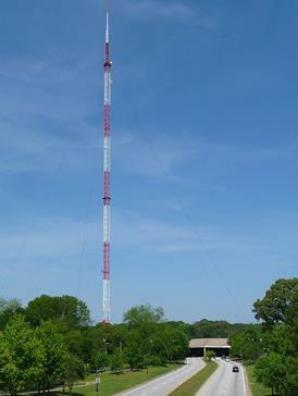
Figure: A MF broadcast monopole antenna with radials buried in the earth. 0.53-1.6 MHz, 50-1500 kW. From Wikipedia.

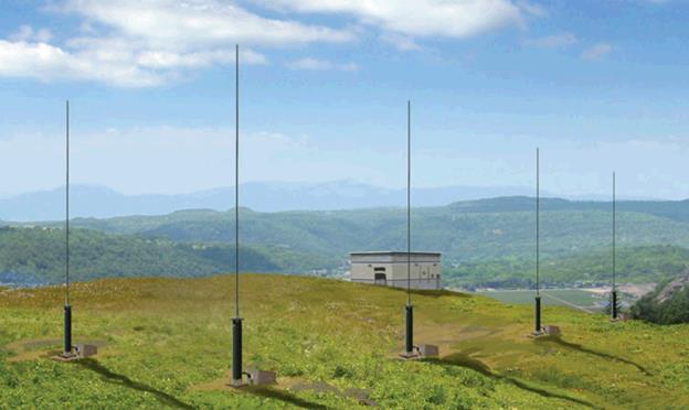
Figure: An array of sleeve monopoles for the TCI 802 DF system operationg at 0.3-30 MHz. From www.tcibr.com

4.3 Shortened Monopoles

- Monopole length reduction methods

Base inductive loading

Middle inductive loading

Top capacitive loading

Top capactive and inductive loading

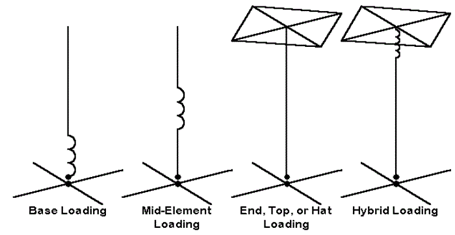
Figure: Monopole length reduction techiques. From webclass.org/k5ijb/antennas/Vertical-antennas.htm.

- Whip antenna: Use a wire of helical shape for size reduction

- Also known as (aka) a normal mode helical antenna.

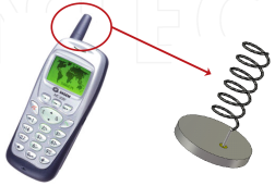
Figure: Whip antennas for (a) 315/433 MHz short range radio [www.embien.com] and (b) 46/49 MHz wireless telephone [L. Huiteman, Progress in Compact Antennas, Chapter 1 Compact Antennas – An Overview]

4.4 Compact Monopole Antennas

1) Meander monopole

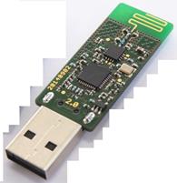
Figure: Meander monopole in a USB Bluetooth dongle. From www.qsl.net/kk4obi/

2) ILA (Inverted L Antenna)

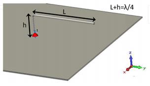
Figure: Inverted L antenna (ILA) [L. Huiteman, Progress in Compact Antennas, Chapter 1 Compact Antennas – An Overview]

3) IFA (Inverted F Antenna)

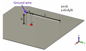
Figure: Inverted F antenna (IFA) [L. Huiteman, Progress in Compact Antennas, Chapter 1 Compact Antennas – An Overview]

- Printed IFA

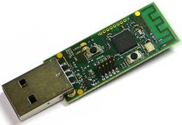
Figure: Printed inverted F antenna. MIMO antenna (left) and (b) USB dongle Bluetooth antenna

4.5 Planar Monopole

Figure: Planar monopole antenna. From N. P. Agrawall et al., "Wide-band planar antennas", IEEE Trans. Antennas Propagat., 46(2), 294-295, 1998.

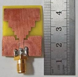
Figure: A wideband plate monopole.

4.6 3D Monopole

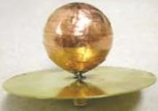
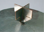
Figure: Various 3D monopole shapes

4.7 Low-profile Monoples

- Small height

Figure: Liu antenna, 425-615 MHz, D = 91 mm, H = 60 mm

Figure: Elsherbini antenna, 0.9-6 GHz, D = 120 mm, H = 17.5 mm

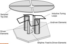
Figure: Goubau antenna, 430-900 MHz, D = 123 mm, H = 43 mm

(d) Nakano antenna, 1-15GHz, D=40mm/H=10mm

(e) Best antenna, 0.55-1.27GHz, D=123mm/H=43mm

(f) Friedman antenna, 325-625MHz, , D=184mm/H=65mm

(g) Ravipati, 0.5-2.7GHz, D=123mm/H=43mm

그림: 높이가 작은 3차원 모노폴

ㅇ Conical monopole/Monocone antenna

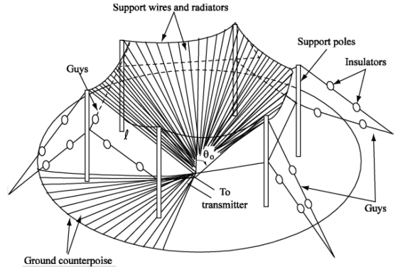
그림: 2-14MHz HF대역 통신용 원뿔 모노폴[Ma & Spies(]. l = 30.6m, a = 0.001m, θ0 = 45º,

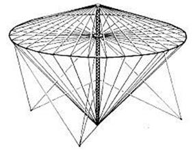
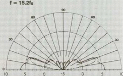
그림: 1.6-30MHz HF monocone antenna, ASC Signal Type 1794 Series GRANGER^TM. 2:1, 40kW-avg, 160kW-peak. Long-range communication via skywave. Short-range communication via groundwave. Low-angle radiation patterns

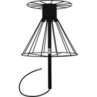
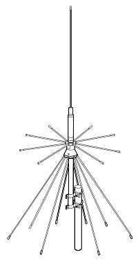
10) Discone 안테나: disc + cone

- Disc는 접지면 역할, cone은 모노폴 역할

- 크기가 큰 경우 (저주파용) 무게를 줄이기 위해 금속면을 wire로 대체

- LF 대역(3-30kHz) 대역에서는 지면에 설치

(a) Zhang, 3-10GHz (b) HYS Co., 0.1-1.1GHz, D=960mm/H=1230mm

(c) Satimo Co., 100-500MHz, D=750mm/H=700mm (d) Telewave Co., 118-2300MHz, D=724mm/H=1092mm

(e) AOR Co., 0.7-6GHz, D=133mm/H=232mm

그림: 디스콘 안테나

- VLF, LF 대역 송신 안테나: 장거리 지표면파 통신, 지상-선박/지상-잠수함 통신, Loran-C 항법

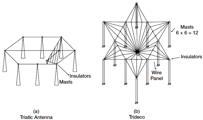
그림: VLF 송신 안테나

- 다이폴과 discone 안테나의 결합

(a) Apex Radio Co., 70-3000MHz, D=630mm/H=1040mm (b) Vimer Co., 25-3000MHz, D=840mm/H=1700mm

(c) Discone(10-30MHz) + cage dipole(3-12MHz) on the USS Iowa

그림: 디스콘과 다이폴이 결합된 안테나

1. 모노폴의 구조

ㅇ 모노폴(monopole) 구조: 아래 그림과 같이 길이 L/2 동작 주파수에서 1/4 파장에 가까운 가는 도선을 완전도체(PEC) 접지판에 수직으로 설치하고 간극(gap) g/2 사이에 전원 인가

L/2 = 모노폴 도선 길이, d = 모노폴 도선 직경, g/2 = 모노폴과 접지판 간극

D = 접지판 직경, t = 접지판 두께

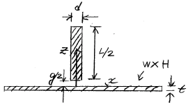
그림: 모노폴 구조

II. 연습문제

1. 수직 다이폴을 이용하여 영상이론을 설명하라.

2. 수평 다이폴을 이용하여 영상이론을 설명하라.

3. 1/2-파장 다이폴과 1/4-파장 모노폴에 대해

1) 구조와 급전점 도시

2) 입력 임피던스 비교

3) 지향도 비교

4. 무한 평면 접지면 위에서 동작하는 모노폴 안테나와 유한 평면 접지면 위에서 동작하는 모노폴의 방사패턴을 비교하라.

5. 다음 안테나 형상을 도시하라.

1) Monopole with radial ground

2) T-antenna

3) Inverted-L antenna

4) Inverted-F antenna

5) Plate monopole

III. 실습

1. 요약

ㅇ 무한접지면 + 수직 1/4 파장 모노폴

ㅇ 무한접지면 + 역 L형 안테나

ㅇ 무한접지면 + 역 F형 안테나

ㅇ 특성확인: 반사계수, 입력임피던스, 이득패턴, 편파특성

2. 실습

2.1 준비

1) 안테나 구조

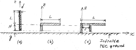
그림 L4.20 (a) 수직 모노폴, (b) 역 L형 안테나, (c) 역 F형 안테나 실습 구조

(치수: d = 4mm, H = 30mm, L = 60mm, S = 4mm(가변), g = 1mm, Discrete port (= delta gap source) 전원 사용

2) 공진주파수 계산

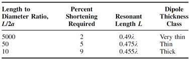
- 다이폴 기준으로 길이 대 직경 비: 2×(30+60)/4 = 45

- 다이폴 공진길이는 아래 표로부터 0.475λ: 2×(30+60) = 0.475λ → λ = 379mm, f = 792MHz

표 L4.1 다이폴 공진길이 [Stutzman]

- 해석 주파수 결정: 400-1200MHz

2.2 시뮬레이션

1) 다이폴

그림 L4.20(a)의 수직 모노폴에 대응되는 다이폴을 그리고 시뮬레이션하라. 다이폴 중심축을 z 축에 일치

a) 안테나 형상

b) 반사계수 plot: Cartesian plot, 400-1200MHz, -30dB to 0dB

c) 중심주파수 = ( )MHz, 대역폭 = ( ) MHz

d) 입력 저항/리액턴스 plot

e) 공진주파수 = ( ) MHz, 공진시 저항 = ( )Ω

f) Gtheta 3D plot (공진 주파수에서)

g) max(Gtheta) = ( )dBi

h) Gphi 3D plot (공진 주파수에서)

i) max(Gphi) = ( )dBi

2) 수직 모노폴

그림 L4.20(a) 수직 모노폴에 대해 위 과정 반복

3) 역 L형 안테나

그림 L4.20(b) 역 L형 안테나에 대해 위 과정 반복

4) 역 F형 안테나

그림 L4.20(c) 역 F형 안테나에 대해 S = 2, 4, 8mm인 경우

a) 안테나 형상

b) 반사계수 plot: 동일 그래프에 Cartesian plot, 400-1200MHz, -30dB to 0dB

2.3 결과요약

Antenna f(MHz) for min (S11) Δf(MHz) for |S11| < -10dB max(Gabs)(dB) R_in(ohm) at resonance

Have-wave dipole

Quarter-wave monopole

Inverted-L antenna