Antenna Design, Monopole Antenna
III. Laboratory Report
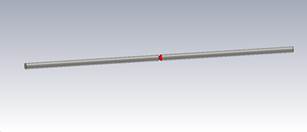
1. A half-wave dipole in free space
Wire
end-to-end length (including the feed gap) = 182
Wire
diameter = 4
Feed
gap = 2
Frequency
range: 400-1200 MHz
Field
monitor: Farfield at the resonant frequency
of each antenna (to be added later)
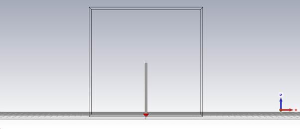
1) Draw
the antenna geometry.
(Using the CST Studio Suite)
(1) Make a PEC cylinder
Modeling, Cylinder icon, ESC key,
Name: solid1, Orientation: Z
Outer radius: 2, Inner radius: 0
Xcenter: 0, Ycenter: 0
Zmin: -182/2, Zmax: 182/2
Material: PEC
(2) Make a feed gap
Modeling, Cylinder icon, ESC key,
Name: solid1, Orientation: Z
Outer radius: 2, Inner radius: 0
Xcenter: 0, Ycenter: 0
Zmin: -2/2, Zmax: 2/2
Material: Vacuum
Next
Shape intersection: Cut away
highlighted shape
3) Add a discrete port source
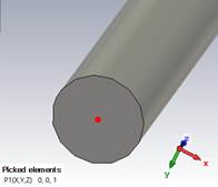
Modeling, Pick Points, Pick Face
Center, select one of the gap faces (double click)
Pick Points, Pick Face Center, select
the other face (double click)
Simulation, Discrete Port
4) Set up the simulation
Define the simulation frequency:
Simulation, Frequency, Min. frequency:
0.4, Max. frequency: 1.2
Set up the field monitor:
Simulation, Field Monitor, E-field,
Frequency, Frequency: 0.74, Apply
Simulation, Field Monitor, H-field and
Surface current, Frequency, Frequency: 0.74, Apply
Simulation, Field Monitor, Far
field/RCS, Frequency, Frequency: 0.74, Apply
5) Define the mesh density if you run
out of a computer memory.
Simulation, Global Properties,
Cells
per wavelength: 5
Cells
per max model box edge: 5
Fraction
of maximum cell near to model: 5
6) Simulation
Simulation, Setup Solver
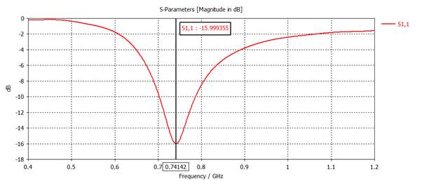
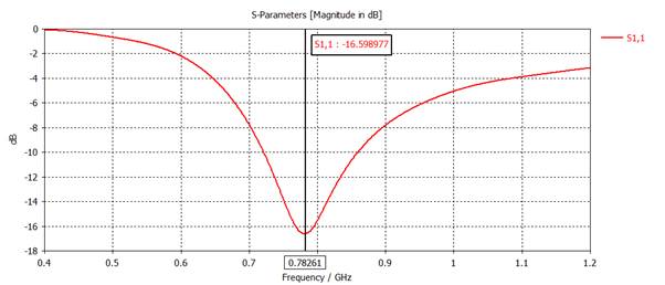
2)
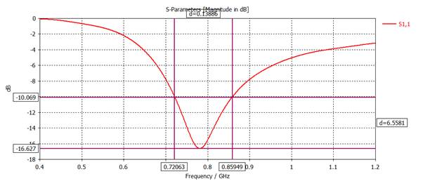
Plot |S11| (dB) and add an 'Axis Marker' to find the frequency for minimum
|S11| (dB).
Center
frequency = 741 MHz
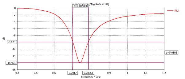
Remove the 'Axis Marker'
and add 'Measure Lines' at |S11| (dB) = -10 dB.
Bandwidth
= 86 MHz
(1)
Add a 'Axis Marker'.
1D Results, S-Parameters, S1,1
RESULT TOOLS - 1D Plot, dB
Mouse right click: show axis marker
(2) Add 'Measure Lines'.
Mouse right click: show measure line
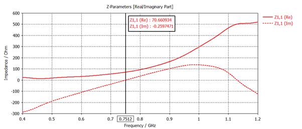
3) Plot Rin and Xin
on a same graph with 'Axis Marker' at Xin = 0. Find the resonant frequency (for
Xin =0) and the resonant resistance (for Xin = 0). Express the dipole length in
the resonant wavelength.
Resonant
frequency = 751 MHz
Resonant
resistance = 67 ohms
Dipole
length in wavelength: wavelength = 300/0.751 = 399, Dipole length = 182/399 =
0.456 wavelength
RESULT TOOLS - 1D Results,
Z Matrix, Z11, 1D Plot, Real/Imag
Mouse right
click: show axis marker
Adjusting: Z1,1(Im) =0
4)
Plot Gtheta in 3D at resonant frequency and
find the maximum gain.
Gmax
= 2.18 dBi
Farfields, farfield (f=0.74) [1], Abs, FARFIELDS - Farfield Plot, Show Structure, 3D
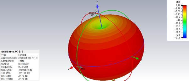
Gmax =2.18dBi
2. A
quarter-wave monopole on an infinite ground plane
Wire
length (except the feed gap) = 90
Wire
diameter = 4
Feed
gap = 1
Frequency
range: 400-1200 MHz
Field
monitor: Farfield at 770 MHz
1) Make
the antenna geometry and plot it in 3D.
(1) Make a monopole wire.
Modeling, Cylinder 아이콘 선택, ESC 키, Name:
solid1, Orientation: Z
Outer radius: 2, Inner radius: 0
Xcenter: 0, Ycenter: 0
Zmin: 1, Zmax: 90
Material: PEC
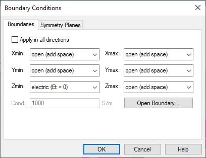
(2) Make an infinite PEC (Et = 0) ground plane on the Zmin
(z = 0) boundary box.
Simulation,
Boundaries, Boundary Conditions, Zmin: choose the electric(Et=0), OK

(3) Define a discrete port.
Modeling, Pick Points, Pick Face
Center, select a face in the gap and double click
Pick Points, Pick Face Center, select the
other face in the gap and double click
Pick Point, Pick point from
coordinates
Simulation, Discrete Port
(4) Setup the simulation.
Set the frequency:
Simulation,
Frequency, Min. frequency: 0.4, Max. frequency: 1.2
Set the field monitor:
Simulation,
Field Monitor, E-field, Frequency, Frequency:0.77,
Apply
Simulation,
Field Monitor, H-field and Surface current, Frequency, Frequency:0.77, Apply
Simulation,
Field Monitor, Far field/RCS, Frequency, Frequency:0.77,
Apply
(5) Simulate.
Simulation, Setup Solver
2)
Plot |S11| (dB) and add an 'Axis Marker' to find the frequency for minimum
|S11| (dB).
Center
frequency = 783 MHz
Remove the 'Axis
Marker' and add 'Measure Lines' at |S11| (dB) = -10 dB.
Bandwidth
= 139 MHz
1D Results, S-Parameters, S1,1
RESULT TOOLS - 1D Plot, dB
Mouse right click: show axis marker
Mouse right click: show measure line
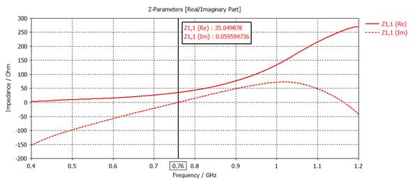
3) Plot Rin and Xin
on a same graph with 'Axis Marker' at Xin = 0. Find the resonant frequency (for
Xin =0) and the resonant resistance (for Xin = 0). Express the dipole length in
the resonant wavelength.
Resonant
frequency = 760 MHz
Resonant
resistance = 35 ohms
Dipole
length in wavelength: wavelength = 300/0.76 = 395, Monopole length = 91/395 =
0.230 wavelength
RESULT TOOLS - 1D Results,
Z Matrix, Z11, 1D Plot, Real/Imag
Mouse right click: show axis marker
Adjusting: Z1,1(Im) =0
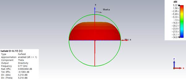
4)
Plot Gtheta in 3D at the resonant frequency
and find the maximum gain.
Gmax
= 5.22 dBi
Farfields, farfield (f=0.77 [1], Abs, FARFIELDS - Farfield Plot, Show Structure, 3D
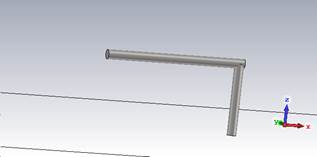
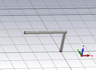
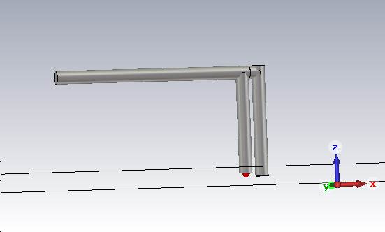
3. An
inverted L antenna on an infinite ground plane
Wire
length: vertical = 30, horizontal = 60
Wire
diameter = 4
Feed
gap = 1
Frequency
range: 400-1200 MHz
Field
monitor: None
1) Make
the antenna geometry and plot it in 3D.
(1) Make
an infinite ground plane.
File, New and Recent, New Template,
Great Project Template, MICROWAVES & RF/OPTICAL,
Antennas, Planar(Patch, Slot, etc,), Time Domain, Next
Frequency Min: 0.4 GHz
Frequency Max: 1.2 GHz
Monitors: not selected
Define at: not entered
Template Name: Inverted
Antenna , Finish
Simulation,
Boundaries, Boundary Conditions, Zmin: choose the
electric (Et=0), OK

(2) Make an inverted L antenna
Modeling, Cylinder, ESC key, Name: solid1,
Orientation: Z
Outer radius: 2 Inner radius: 0.0
X center: 0 Y center: 0
Z min: 1 Z max:31
Material: PEC
Modeling, Cylinder, ESC key, Name: solid2,
Orientation: X
Outer radius: 2 Inner radius: 0.0
Y center: 0 Z center: 31
X min: -58 X max: 2
Material: PEC
(3) Make a discrete port.
Modeling, Pick Points, Pick Face
Center, select a face in the gap and double click.
Modeling, Pick Points, Pick Point From
Coordinates
Enter 3D point, X:0,
Y: 0, Z:0 OK
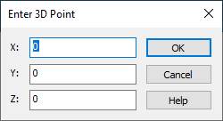
Simulation, Discrete Port, OK
Simulation, Setup Solver
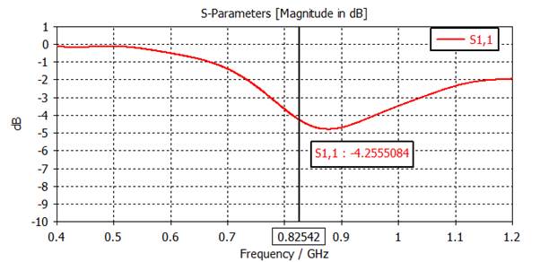
2) Plot |S11| (dB).
1D Results, S-Parameters, S1,1
RESULT TOOLS - 1D Plot, dB
Right click, Plot Properties, Auto
range deselected
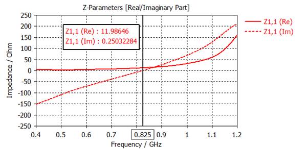
3) Plot Rin and Xin
on a same graph with 'Axis Marker' at Xin = 0. Find the resonant frequency (for
Xin =0) and the resonant resistance (for Xin = 0).
Resonant frequency = 825
MHz
Resonant
resistance = 12 ohms
RESULT TOOLS - 1D Results,
Z Matrix, Z11, 1D Plot, Real/Imag
Mouse right click: show axis marker
Adjusting: Z1,1(Im) =0
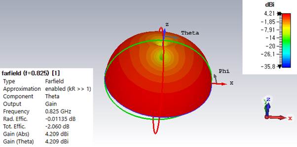
4) Plot Gtheta in 3D
at the resonant frequency and find the maximum gain.
Gmax = 4.21 dBi
Farfields, farfield (f=0.825)
[1], Theta,
Far Field
Properties, Plot mode, plot mode and scaling, choose the gain (IEEE)
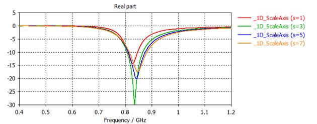
4. An inverted F antenna on an infinite ground
plane
Wire length: vertical = 30, horizontal = 60
Wire diameter = 4
Feed gap = 1
Frequency range: 400-1200 MHz
Field monitor: Farfield at
800 MHz
Shorted-wire to feed-wire gap (S) = 1, 2, 4, 8
(Use the parameter sweep)
1) Draw the antenna geometry.
(1) Make a template. Define an infinite ground plane.
File, New and Recent, New Template, Great Project
Template, MICROWAVES & RF/OPTICAL,
Antennas, Planar(Patch, Slot, etc,), Time Domain, Next
Frequency Min:
0.4 GHz
Frequency Max:
1.2 GHz
Monitors: check the E-field, H-field, Farfield, Power loss
Define at: 0.8 GHz, Next
Template Name: Inverted Antenna , Finish
Simulation, Boundaries, Boundary Conditions, Zmin: choose the electric(Et=0),
OK
Modeling, 고리 실린더 (Cylinder) 선택, ESC 키, Name:
solid1, Orientation: Z
Outer radius: 2 Inner radius: 0.0
X center: 0 Y center: 0
Z min: 1 Z max:31
Material: PEC
Modeling, 고리 실린더 (Cylinder) 선택, ESC 키, Name:
solid2, Orientation: X
Outer radius: 2 Inner radius: 0.0
Y center: 0 Z center: 31
X min: -58 X max: 2
Material: PEC
Modeling, 고리 실린더 (Cylinder) 선택, ESC 키, Name:
solid3, Orientation: X
Outer radius: 2 Inner radius: 0.0
Y center: 0 Z center: 31
X min: 2 X max: 4+s
Material: PEC
Modeling, 고리 실린더 (Cylinder) 선택, ESC 키, Name:
solid4, Orientation: Z
Outer radius: 2 Inner radius: 0.0
X center: 4+s Y center: 0
Z min: 1 Z max:33
(3) Make a discrete port
Modeling, Pick Points, Pick Face
Center, gap 한면에 마우스 위치후 더블클릭

Modeling, Pick Points, Pick Point From
Coordinates
Enter 3D point, X:0,
Y: 0, Z:0 OK
Simulation, Discrete Port, OK
(4) Simulate.
Simulation, Setup Solver, Start
2) Plot |S11| (dB) for five cases on a same graph.
(1) Setup a parameter sweep.
Simulation, Setup Solver, Time Domain
Solver Parameters, Par. Sweep,
New Sequence, New Parameter, Parameter
Sweep Parameter
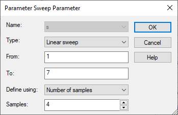
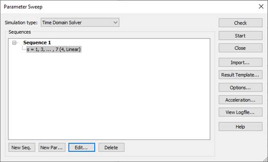
close
(2) Setup the output plot.
Post-Processing, Result Templates
Tools, General 1D, choose the 0D or 1D result from 1D Result (Rescale,
Derivation, etc)
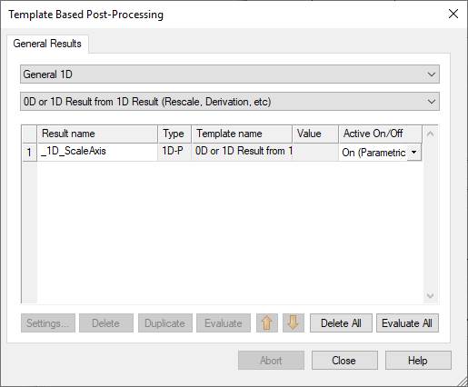
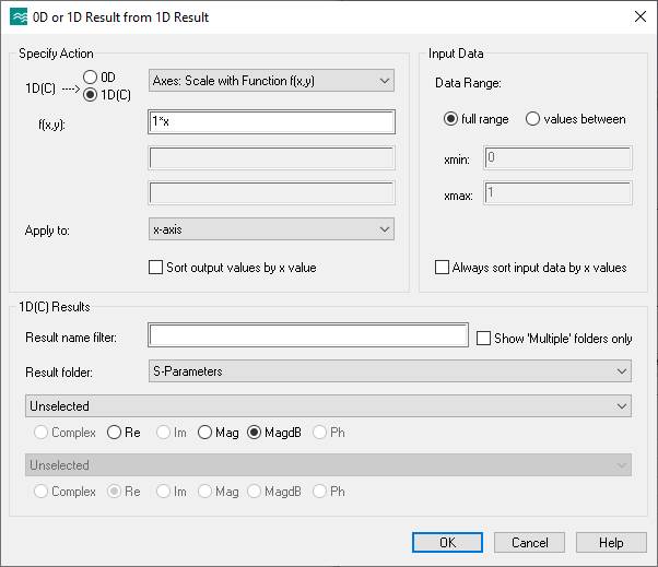
Ok
(3) Do the parameter sweep.

Evaluate All
Simulation, Setup Solver, Start
0D or 1D result.
(4) Plot |S11| (dB).
1D Results, S-Parameters, S1,1
RESULT TOOLS - 1D Plot, dB