Microwave Engineering 01, Python Coding

1. Online study material

Tutorials Point 'Learn Python': https://www.tutorialspoint.com/python/index.htm

2. Use Online Python

- Access https://www.online-python.com/

- Copy or write down your code in the upper window of 'Online Python'.

- Click [Run]

- In the lower window, enter your data.

- Program output will be displayed in the lower window.

- To copy the text in the lower window, click [Stop], click the left top icon

- Go to your document, then press Ctrl + V

(참고)

ㅇ 상단창(소스코드창) 상단에 배치된 아이콘 메뉴 의미

상단좌측 아이콘 4개: Open file From Disk, Save File to Disk, Undo, Redo

상단우측 아이콘 3개: Change Theme, About Site, Settings

ㅇ 하단창(입출력창) 좌측 아이콘 메뉴 5개의 의미

Copy to clipboard: 출력창 내용을 클립보드에 copy (다음에 Ctrl+v로 문서에 삽입)

Download: 출력창 내용을 txt 파일로 컴퓨터로 다운로드

Clear: 출력창 내용 지움

Smart terminal: >>>가 표시되고 interpreter 모드. Python를 1줄씩 실행. help(print)

와 같이 help 표시

Expand/Collapse: Expand = 출력창만 전체화면에 표시, Collapse: 위창, 아래창 동시표시

3. 코딩실습

3.1 Example 1: Transmission line. Calculate Z0, γ using R, L, G, and C.

1) 문제

Input: R, L, G, C of a transmission, f

Output: Z0, γ

2) 수식

R in ohm/m

L in H/m

G in S/m

C in F/m

Z0 in ohm

Re(γ) in Np/m

Im(γ) in rad/m

3) 코딩

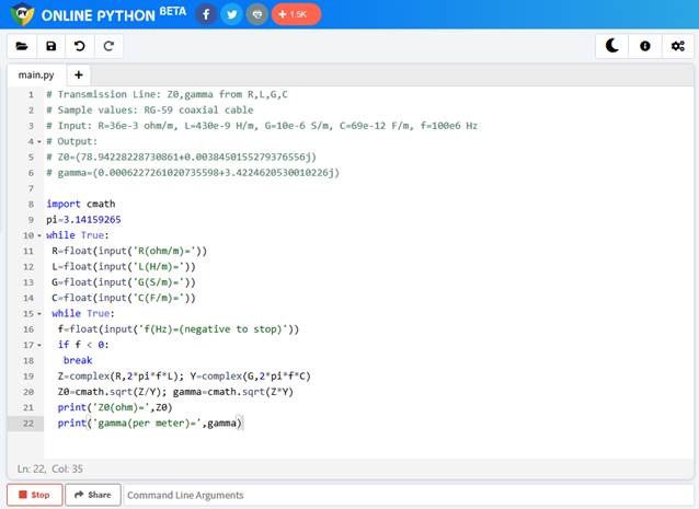
# MW-01-Python-Ex1

# Transmission Line: Z0, gamma from R, L, G, C, f

# Sample values: RG-59 coaxial cable

# Input: R=36e-3 ohm/m, L=430e-9 H/m, G=10e-6 S/m, C=69e-12 F/m, f=100e6 Hz

# Output:

# Z0=(78.94228228730861+0.0038450155279376556j)

# gamma=(0.0006227261020735598+3.4224620530010226j)

import cmath

pi=3.14159265

while True:

R=float(input('R(ohm/m)='))

L=float(input('L(H/m)='))

G=float(input('G(S/m)='))

C=float(input('C(F/m)='))

while True:

f=float(input('f(Hz)=(negative to stop)'))

if f < 0:

break

Z=complex(R,2*pi*f*L); Y=complex(G,2*pi*f*C)

Z0=cmath.sqrt(Z/Y); gamma=cmath.sqrt(Z*Y)

print('Z0(ohm)=',Z0)

print('gamma(per meter)=',gamma)

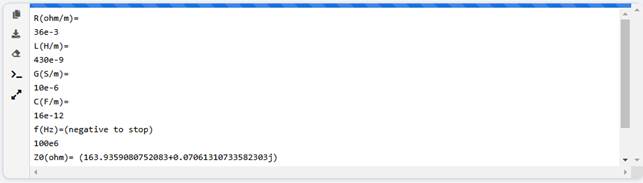
4) 코드 수행결과

R(ohm/m)=

36e-3

L(H/m)=

430e-9

G(S/m)=

10e-6

C(F/m)=

69e-12

f(Hz)=(negative to stop)

100e6

Z0(ohm)= (78.94228228730861+0.0038450155279376556j)

gamma(per meter)= (0.0006227261020735598+3.4224620530010226j)

f(Hz)=(negative to stop)** Process Stopped **

Press Enter to exit terminal

3.2 Example 2: Transmission line. Calculate R, L, G, and C from Z0 and γ

1) 문제

Input: Z0, γ

Output: R, L, G, C

2) 수식

3) 코딩

# EM-01-Python-Ex2: R, L, G, C from Z0, γ and f

# Input: Z0 = 79 + 3.8e-3j, gamma=6.2e-4+3.4j, f=100e6

# Output:

import cmath

pi=3.14159265

while True:

Z0=complex(input('Z0(ohm)='))

gamma=complex(input('gamma(per meter)='))

f=float(input('f(Hz)='))

w=2*pi*f

temp=gamma*Z0 ; R=temp.real ; L=temp.imag/w

temp=gamma/Z0 ; G=temp.real ; C=temp.imag/w

print('R(ohm/m)=',R)

print('L(H/m)=',L)

print('G(S/m)=',G)

print('C(F/m)=',F)

4) 코드 수행결과

Z0(ohm)=

79+3.8e-3j

gamma(per meter)=

6.2e-4+3.4j

f(Hz)=

100e6

R(ohm/m)= 0.03606

L(H/m)= 4.27490181383e-07

G(S/m)= 9.918282303601987e-06

C(F/m)= 6.849706343446908e-11

Z0(ohm)=** Process Stopped **

Press Enter to exit terminal

3.3 Example 3: 복소수 계산

(참고) Python에서 복소수 연산

ㅇ 표기: 1+2j, 1.+1.j, 2j

ㅇ 입력시 괄호 없이 1+2j와 같이 입력

ㅇ 출력시 괄호가 사용됨 (실수, 허수 모두 있을 때)

2j

(1+2j)

ㅇ 실수부와 허수부는 실수 규칙을 따름.

ㅇ 복소수 지정

z=3+2j

z=complex(3,2)

ㅇ 복소수 연산

4칙연산: + - * / **

z1+z2, z1-z2, z1*z2, z1/z2

z1**2, pow(z, 2), z1**z2

z.real

z.imag

z.conjugate()

z=complex(x, y)

z=complex(2, 4)

z=complex(2) # z=2+0j

ㅇ 복소수 라이브러리 함수

from cmath import *

polar(z): a tuple value

zm=polar(z)

zm[0] : mag(z)

zm[1] : phase(z)

rect(r, phi) : a complex value

exp(z), phase(z), abs(z), log(z, [base]), log10(z), sqrt(z)

acos(z), asin(z), atan(z), cos(z), sin(z), tan(z)

acosh(z), asinh(z), atanh(z), cosh(z), sinh(z), tanh(z)

ㅇ Tuple: 항목값 변경 불가, 변경가능한 것은 list

t1 = ()

t2 = (1,)

t3 = (1, 2, 3)

t3[0] # t3의 첫번째값 1

len(t3) # t3의 요소수 4

t3*3

t4 = 4, 5, 6

t3+t4 # (1,2,3,4,5,6)

t5 = ('a', 'b', ('ab', 'cd'))

t6=t3+t4

t6[1:4] # (2,3,4,5)

t6[1:] # (2,4,4,5,6)

t6[:4] # (1,2,3,4,5)

1) 문제

복소수 z1과 z2를 입력받아 z3 = z1*z2, z4=z1/z2를 실수/허수, 크기/위상(radian)으로 표시

2) 수식

3) 코딩

# MW-01-Python-Ex3: Complex calulation

from cmath import * # Use the complex math library in Python

while True:

z1=complex(input('z1='))

z2=complex(input('z2='))

z3=z1*z2; z4=z1/z2

zp3=polar(z3); zp4=polar(z4)

z3arg=zp3[1]*180/3.14159

z4arg=zp4[1]*180/3.14159

print('z3=',z3,'z3(polar)=',zp3,'arg(z3)(deg)=',z3arg)

print('z4=',z4, 'z4(polar)=',zp4,'arg(z4)(deg)=',z4arg)

4) 코드 수행결과

z1=

1+2j

z2=

3+4j

z3= (-5+10j) , z3(polar)= (11.180339887498949, 2.0344439357957027) , arg(z3)(deg)= 116.56514963544781

z4= (0.44+0.08j) , z4(polar)= (0.4472135954999579, 0.17985349979247828) , arg(z4)(deg)= 10.304855172904833

z1=** Process Stopped **

Press Enter to exit terminal

3.4 Example 4: R, L, C serie circuit impedance

1) 문제

R, L, C, f 가 주어진 경우 RLC 직렬회로와 RLC 병렬회로의 임피던스를 계산하라.

2) 수식

R in Ω (Ohm)

L in H (Henry)

C in F (Farad)

ω in rad/s

f in Hz (Herz)

3) 코딩

# MW-01-Python-Ex4: RLC series and parallel circuits

pi=3.141593

while True:

R=float(input('R(ohm)='))

L=float(input('L(uH)='))

C=float(input('C(uF)='))

f=float(input('f(Hz)='))

w=2*pi*f

Zs=complex(R, w*L*1e-6-1/(w*C*1e-6))

Zp=1/complex(1/R, w*C*1e-6-1/(w*L*1e-6))

print('Z(series)=', Zs)

print('Z(parallel)=', Zp)

4) 코드 수행결과

R(ohm)=

100

L(uH)=

20

C(uF)=

50

f(Hz)=

1e6

Z(series)= (100+125.66053690148915j)

Z(parallel)= (1.0132629437904996e-07-0.0031831791384774404j)

R(ohm)=** Process Stopped **

Press Enter to exit terminal